ComputeGradB and Autodiff
This section documents the ComputeGradB pathway in virtual_casing_jax and
how it is used for JAX-based automatic differentiation. The goal is to make the
gradient of the external magnetic field on the surface available with
high-order singular quadrature and end-to-end differentiability.
Overview
ComputeGradB returns the on-surface gradient of the external field
on the surface Gamma where the total field B is prescribed. This is the
operator needed in single-stage optimization when objectives depend on
B and its spatial derivatives. Typical examples include:
derivatives of
|B|orB^2on the surfacesensitivities of
B \cdot nor normal field errorpenalty terms involving
\nabla Bfor smoothness or stability proxies
Equations (from the BIEST formulation)
Let \sigma = \mathbf{B}\cdot\mathbf{n} and \mathbf{K} = \mathbf{n}\times\mathbf{B}.
For targets on Gamma the virtual casing formula gives [MCO2019]:
where G is the Laplace single-layer potential:
Taking a spatial derivative yields the on-surface field gradient:
Here \partial_i\partial_j G is the hypersingular Laplace kernel,
implemented in BIEST and ported to JAX as LaplaceFxd2U. The explicit
second derivative kernel used in this code base is:
matching the formulation in [MCO2019].
Implementation Map
The high-level call VirtualCasingJAX.compute_external_gradB implements:
Complete and resample the surface field. The input
B0is completed over the full toroidal period and resampled to the quadrature grid.Form surface densities:
\[\mathbf{K} = \mathbf{n} \times \mathbf{B}, \qquad \sigma = \mathbf{B} \cdot \mathbf{n}.\]Evaluate hypersingular operators:
laplace_fxd2_u_eval_vec_singularcomputes\partial_i\partial_\ell G[K_m]on the target grid.laplace_fxd2_u_eval_singularcomputes\partial_i\partial_k G[\sigma]on the target grid.
Assemble the curl for the vector term:
\[(\nabla \times G[\mathbf{K}])_k = \partial_{k_1} G[K_{k_2}] - \partial_{k_2} G[K_{k_1}],\]with cyclic indices
(k, k_1, k_2).
The implementation mirrors the C++ ComputeGradB path, including the
same quadrature order, patch selection, and singular corrections.
Reference Mapping
The following functions align with the reference C++ API:
VirtualCasingJAX.compute_external_gradB→VirtualCasing::ComputeGradBext(C++)VirtualCasingJAX.compute_internal_gradB→VirtualCasing::ComputeGradBint(C++)VirtualCasingJAX.compute_external_gradB_offsurf→VirtualCasing::ComputeGradBOffSurf(C++ local parity extension)
The port preserves:
kernel normalizations (
1/(4*pi)),patch/POU construction,
hedgehog order,
grid placement for half-period symmetry.
Singular Quadrature (POU + Polar + Hedgehog)
The on-surface operators are hypersingular. The JAX port uses the same three-part strategy as BIEST [MCO2019]:
Partition of Unity (POU) to localize the singular region.
Polar interpolation for near-singular contributions.
Hedgehog quadrature to evaluate the hypersingular terms at the target.
These steps are implemented in laplace_fxd2_u_eval_singular and
laplace_dx_u_eval_singular. The combination produces a stable
O(h^{p})-accurate on-surface limit that matches the reference
implementation.
Autodiff Strategy
Naive autodiff through the singular quadrature stack is both slow and
numerically fragile. Instead, virtual_casing_jax uses a custom JVP
that contracts the analytically defined surface gradient with a target
perturbation:
This is implemented in
VirtualCasingJAX.compute_external_B_autodiff using jax.custom_jvp.
The JVP calls compute_external_gradB and applies:
This provides exact on-surface derivatives consistent with the C++
ComputeGradB operator, and it avoids differentiating through the
singular correction machinery.
For off-surface GradB, no custom JVP is used. The kernels are smooth off the surface, so JAX can differentiate through the direct quadrature if needed, though this is currently not JIT-friendly when adaptive refinement is enabled.
Performance and Memory Controls
The GradB path exposes several knobs to balance speed and memory:
chunk_sizeandtarget_chunk_sizeenable 2D tiling over sources and targets. This reduces large temporaries in the hypersingular kernels.remat=Trueactivatesjax.checkpointon the singular correction to reduce saved intermediates during autodiff.pou_dtype="auto"(or"float32") casts POU/polar tables to float32 while keeping the final accumulation in float64.patch_dtype="auto"(or"float32") casts the patch interpolation weights and patch gathers inside the singular correction to float32, reducing the largest intermediate tensors while preserving output precision.interp_block_size="auto"(or an integer) blocks the polar interpolation in the singular correction. This reduces temporary memory at the cost of additional loop overhead.
These options are available on compute_external_gradB /
compute_internal_gradB and their JIT wrappers.
Internal and Off-Surface GradB
The internal gradient uses the same on-surface hypersingular operators, but with the sign flipped:
This matches the reference implementation in virtual-casing and is
validated in parity tests. Note that the on-surface hypersingular evaluation
uses the same quadrature orientation for internal and external limits, which
is consistent with the C++ behavior.
For off-surface targets, the jump term is absent and the gradient is evaluated using direct quadrature (no singular correction):
with \mathbf{K} = \mathbf{n}\times\mathbf{B} and
\sigma = \mathbf{B}\cdot\mathbf{n} defined on the source surface.
The JAX implementation optionally upsamples the source grid using the
same LaplaceDxU self-test used by the adaptive off-surface field
evaluation. The current parity path mirrors the reference C++ off-surface
GradB implementation, which uses the base resampled grid (no adaptive
refinement).
Parity and Validation
Parity means the JAX and C++ implementations agree for identical inputs to within the specified tolerances. We use the relative L2 error:
The parity suite includes:
tests/test_virtual_casing_gradb_parity.py(ComputeGradB parity)tests/test_autodiff_gradb_parity.py(autodiff JVP parity)tests/test_virtual_casing_gradbint_parity.py(internal GradB parity)tests/test_virtual_casing_offsurf_parity.py(off-surface B/GradB parity)
The following figures show parity on the SIMSOPT VMEC case.
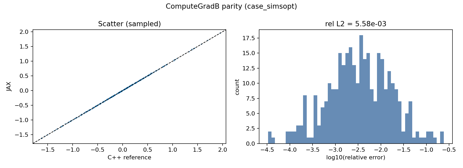
ComputeGradB parity: JAX vs C++ scatter (left) and log10 relative error distribution (right) for the SIMSOPT VMEC case.
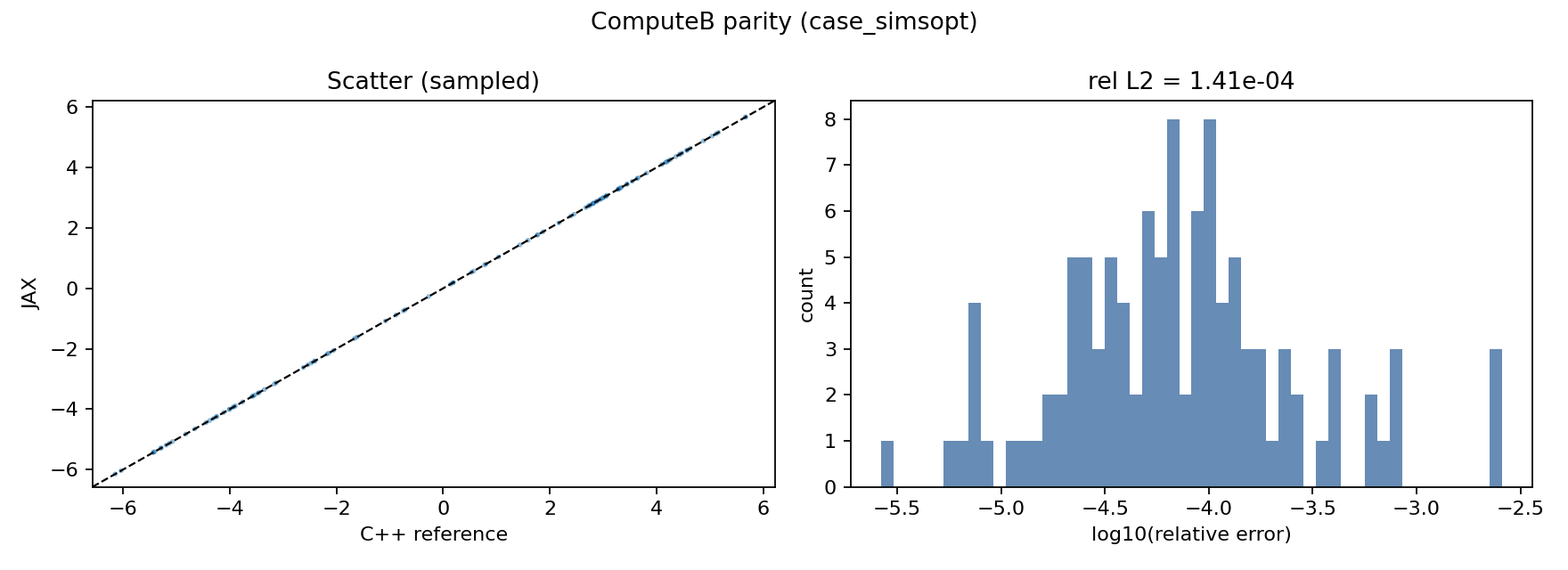
ComputeB parity: JAX vs C++ scatter (left) and log10 relative error distribution (right) for the SIMSOPT VMEC case.
Where GradB Is Used in Optimization
ComputeGradB enables gradients of common physics objectives. Examples:
Field magnitude penalties:
\[f = \int_\Gamma |B|^2\, d a, \qquad \nabla f \propto \int_\Gamma 2\,\mathbf{B}\cdot (\nabla \mathbf{B})\, d a.\]Normal-field control:
\[f = \int_\Gamma (\mathbf{B}\cdot\mathbf{n})^2\, d a.\]The derivative involves
\nabla \mathbf{B}and the geometry Jacobian.Single-stage finite-beta optimization:
\nabla \mathbf{B}couples to VMEC state sensitivities and allows a fully differentiable pipeline without finite-differencing.
Limitations (Current)
The remaining gaps before declaring a complete port include:
A fully functional API that treats the surface coordinates as differentiable inputs (needed for shape-derivative workflows).
End-to-end JIT-compatible adaptive loops (off-surface refinement is a Python loop today).
Additional large-scale validation cases beyond the parity harnesses.